Tutorial: Enzymatic behaviour
Before attempting this section read:
Chapter 5: Detour Enzymes as catalysts
Chapter 7: Detour Allosteric enzymes
Enzymatic tests are frequently used to determine metabolite concentrations and the activity of enzymes in blood tests. In this experiment, we will determine blood glucose concentration by an enzymatic test. Fasting glucose in humans lies between 4-5 mM. After a carbohydrate-rich meal blood glucose can go up to 8 mM in a normal person but can be well above 10 mM in a diabetic person. To remove glucose after a meal the body uses it to fill up glycogen stores in muscle and liver and uses glycolysis to produce energy, particularly during exercise. Any excess glucose that remains unused is converted into fat in liver and transported to adipose tissue (these topics are covered in the lectures).
Enzymatic tests use a combination of enzymes to convert a metabolite into a product that can be detected by a spectrophotometer. In many tests the detectable product is generated by a redox reaction, for example by producing NADH (or NADPH). We will use the first step of glycolysis and the first step of the pentose-phosphate pathway (discussed in the lectures) to convert glucose to 6-phosphogluconolactone. The reactions are as follows:
D-glucose + ATP → Glucose-6-phosphate + ADP
(enzyme: Hexokinase)
Glucose-6-phosphate + NADP+ –> 6-phosphogluconolactone + NADPH + H+
(enzyme: Glucose-6-phosphate dehydrogenase)
The formation of NADPH can be detected by an increase of absorbance at 340 nm (Fig. 1). The optimal pH value for the measurement is 7.7. The free energy of the hexokinase reaction is ΔG°’ –16.7 kJ/mol, the free energy for glucose-6-phosphate dehydrogenase is –12 kJ/mol. As a result, the equilibrium of the combined reaction will strongly favor the products and convert glucose almost completely. Both hexokinase and G-6-P-DH require Mg2+ ions to be active. The magnesium-dependence is mainly caused by the fact that ATP forms a complex with Mg2+ in solution.
The glucose-6-phosphate dehydrogenase reaction produces reduced NADPH, which has a distinct absorbance at 340 nm (Fig. 1). The increase of this absorbance is used to determine the amount of NADPH produced, which is linked stoichiometrically to the amount of glucose.
The amount of NADPH produced by the reaction can be calculated using the molar extinction coefficient of NADPH (ε = 6.31 mM-1cm-1) and the Beer-Lambert law: Absorbance = ε x c (mM) x length of cuvette (cm). NADPH is produced because glucose-6-phosphate is oxidised in this test transferring two electrons to NADP+.
Exercise No 1: Determine the reaction rate
In this virtual experiment we follow the generation of NADPH as in Lab 1. When you add glucose to the cuvette it will be converted via the two enzymes into an equivalent amount of NADPH.
Thus, you can calculate the final optical density in your assay.
This time you make a different experiment. You assemble the same reaction, but use lower glucose concentrations (10 µM, 20 µM, 50 µM, 100 µM, 200 µM, 1000 µM) and follow the reaction over time.
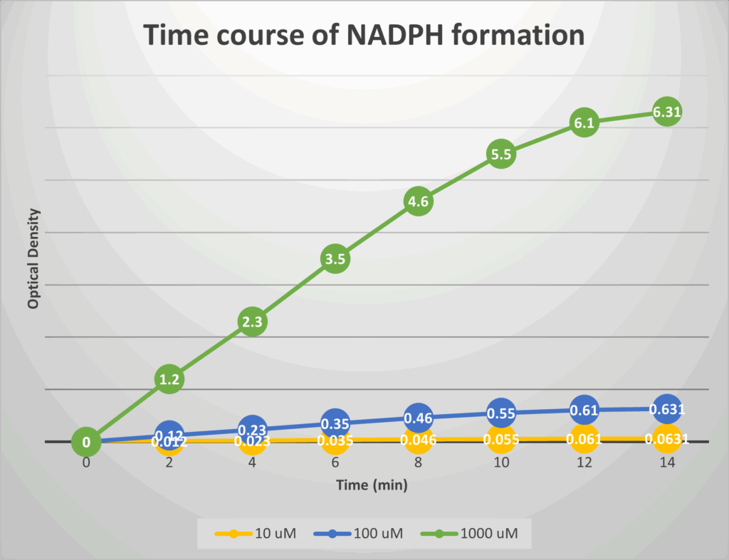
What do you think the time course would look like?
Draw curves by hand on a piece of paper for glucose concentrations of: 10 µM, 100 µM, and 1000 µM.
The curves do not need to be exact but should have the right shape and relative end points.
Calculate the expected endpoint using the Lambert-Beer law.
Optical density = ε x c (mM) x length of cuvette (cm)
The length of the cuvette is 1 cm. The extinction coefficient of NADPH is ε = 6.31 mM-1cm-1 (units in mM/L)
For 10 uM the OD=0.0631
For 100 uM the OD=0.631
For 1000 uM the OD=6.31
How would you determine the rate of each reaction?
The slope at the beginning of the time course equals the rate of the reaction.
Think of the ratio of hexokinase to glucose-6-phosphate dehydrogenase in your assay. In what ratio (qualitatively) would you add the two enzymes to measure the rate of hexokinase?
The indicator reaction (glucose-6-phosphate dehydrogenase) should be much faster than hexokinase. Otherwise, we would measure the velocity of the indicator reaction.
Exercise No 2: Plot your data
In exercise 1 you have determined the reaction rate at three different concentrations. You repeat the experiments with more concentrations and now you want to plot your data. You list the substrate concentrations and the corresponding reaction rates (initial slopes) as listed below.
| Substrate concentration (μM) | Reaction rate (v) (μmol/min per mg protein) |
| 10 | 9 |
| 20 | 18 |
| 50 | 33 |
| 100 | 50 |
| 200 | 65 |
| 500 | 85 |
| 1000 | 91 |
Plot the data on a separate sheet.
Draw the plot and estimate Km and Vmax and write the numbers on a sheet of paper.
Km 100 uM
Vmax 100 umol/min per mg protein
Question
How does your graph look like?
Exercise No 3: Linearised plot
Depending on your answer you may have noted that it is difficult to estimate Km and Vmax with good accuracy from a curve.
We can do this computationally, but for the human eye a straight line is easier.
Linearised versions of the Michaelis-Menten Diagram have been developed, the most well-known is the Lineweaver-Burke Diagram.
Linearisation according to Lineweaver-Burk uses the inverse of the Michaelis-Menten formula:
1/v=(1/V)+(Km/V)∗1/[S]
Now plot your data using 1/v (y-axis) versus 1/S (x-axis) and see how the graph looks like.
In this diagram the intersection with the x-axis will give you 1/Km, the intersection with the y-axis will give you 1/Vmax.
You can calculate Km and Vmax using the linear equation shown in the graph below, by setting x=0 or y=0.
How does your data table look like?
| Substrate concentration (μM) | Reaction rate (v) (μmol/min per mg protein) | 1/v | 1/S |
| 10 | 9 | 0.11 | 0.1 |
| 20 | 18 | 0.056 | 0.05 |
| 50 | 33 | 0.03 | 0.02 |
| 100 | 50 | 0.02 | 0.01 |
| 200 | 65 | 0.015 | 0.005 |
| 500 | 85 | 0.012 | 0.0002 |
| 1000 | 91 | 0.011 | 0.0001 |
Question
How does your graph look like?
What are the values for Km and Vmax?
Km = 94.6 μmol/L
Vmax = 96.6 μmol/min per mg protein
Exercise No 4: Compare enzymes
Below are the Substrate-concentration-versus-reaction-rate diagrams of 3 enzymes.
You can setup your own Excel sheet to follow the tutorial:
Setup a field like this:
| Enz 1 | Km | 60 | Vmax | 100 | ||
| Enz 2 | Km | 500 | Vmax | 100 | ||
| Enz 3 | K0.5 | 7400 | Vmax | 185 | Subunits | 1.77 |
Setup a row with substrate concentrations 0,20,50,100,200,500,1000,2000,3500,5000,7000,10000
and underneath 3 empty rows for your enzymes.
Setup calculations for each free field of enzyme 1 and enzyme 2:
Field value = Vmax * [Substrate concentration]/(Km + [Substrate concentration])
Drag your formula across all rows.
Setup calculations for each free field of enzyme 3 (n= subunit input field):
Field value = Vmax * [Substrate concentration^n]/(Km^n + [Substrate concentration^n])
Drag your formula across all rows.
Select all output-fields (including the concentrations) and use Insert>Chart>Scatter (with lines).
Your graph should now look like this:
Describe the enzymes in terms of their kinetic properties. What is the same and what are the differences. Can you observe certain characteristics or behaviour?
All enzymes have the same Vmax.
Enzyme Blue is a high-affinity enzyme.
Enzyme Orange is a low-affinity enzyme.
Enzyme Grey is an allosteric enzyme.
Draw on paper or generate and Excel sheet that plots the reaction rate at concentrations (uM): 0, 20, 50, 100, 200, 500, 1000, 2000, 3500, 5000, 7500 and 10000 for enzyme orange (Km of 2000 uM and Vmax of 100).
Place a vertical line at the position where Enzyme Orange has its Km-value (remember enzyme Orange has the same Vmax as enzyme Blue). What happens to the Km-value when the Vmax of enzyme Orange is increased from 100 to 200 and to 400?
Does a change of Vmax affect the Km-value?
The Km-value does not change.
Start from the kinetic behavior of Enzyme Orange (Vmax = 100, Km = 2000 uM).
What happens to the curve when you set the Km to 500 uM and 10000 uM?
As the Km increases, higher substrate concentrations are needed to reach Vmax.
Have a look at the curve with a Km of 10000 uM. Can you estimate the Vmax with precision?
Yes, the Km is at 0.5 x Vmax. At the Km the reaction rate is 50, so Vmax must be 100.
Allosteric enzymes are multimeric and the subunits influence each other. Increase the number of subunits from 1 to 4 and look at the response of the enzyme to changes of substrate concentration.
Note: The response to changes of the number of subunits is idealised. For instance, the real behaviour of an enzyme with two subunits would look more like 1.5 or 1.6 (which you can test) an enzyme with three subunits would look like 2.5 etc.
How does the curve change?
As the number of subunits increase the sigmoidity of the curve increases.
Exercise No. 4:
Make Enzyme Orange glukokinase (K0.5=7400 uM, subunits = 1.77, Vmax = 185) and make enzyme blue hexokinase (Km 60 uM, Vmax = 100).
Graph on back side
Your graph should look like this.
Determine the change of reaction rate when glucose concentration increases from 4 mM to 8 mM (e.g. after a meal).
- Which enzyme responds more dynamically to the change?
- Where is this enzyme found and why?
Hexokinase increases from 98 to 99.
Glucokinase increase from 46 to 99. Considering that the Vmax is almost twice as high the change is 25 times more dynamic.
Glucokinase is found in the liver and pancreas, the two organs where metabolism responds to glucose intake.
You can use the graph below to play around with Km, Vmax and n values and compare enzymes. For a standard enzyme set n=1.


